Excel pie chart group data

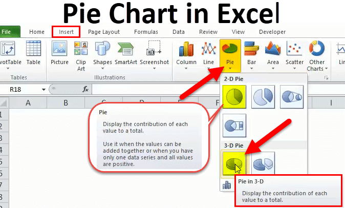
Lets see how to create Pie of Pie chart in Excel. In the charts group Select the pie chart button Click on pie chart in 2D chart section.

Make Pie Graphs And Frequency Distributions In Excel Categorical Data Youtube

Define a pie chart and suggest how to make it in Excel.

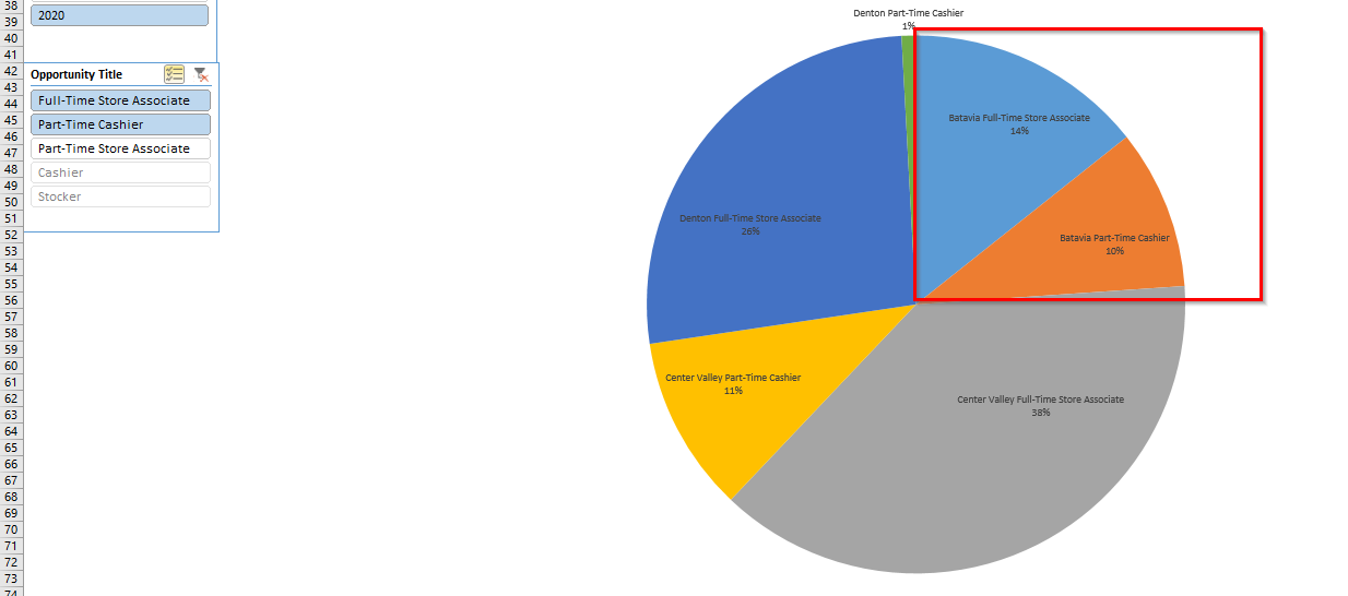
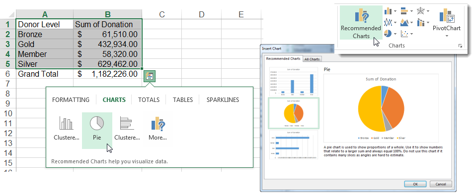
. Select the entire dataset Click the Insert tab. When the user selects a date you want the Items property of the pie chart to respond by filtering out only the data from that date. A pie chart sometimes called a circle chart is a useful tool for displaying basic statistical data in the shape of a circle each section resembles a slice of pie.

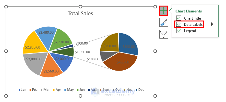
When I insert into a pie chart it gives. Select the data click Insert tab chose pie chart ribbon Pie of pie chart as shown below. Adding Data Labels The default pie chart inserted in the above section is- From this.

In columns or rows. It is a circular chart consisting of slices. Prepare a table and group data there.

First select the dataset and go to the Insert tab from the ribbon. After that click on Insert Pie or Doughnut Chart from the Charts group. In the Charts group click on the Insert Pie or Doughnut.

Column bar line area surface and radar charts. Column bar line area surface or radar chart. Select data and under Insert option in toolbar In Column select first option.

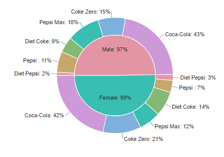
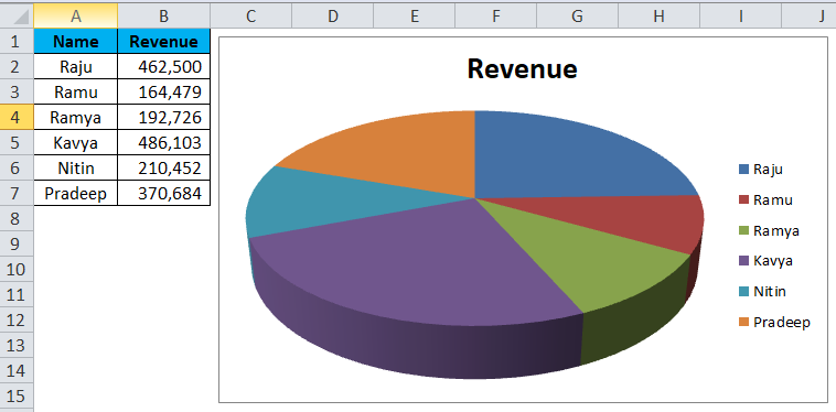
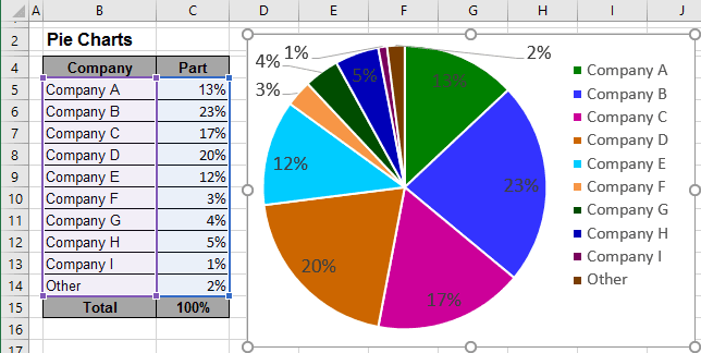
What is Pie Chart in Excel A Pie Chart shows the percentage contribution of different data categories in the whole pie. Select the cell range A1B7 go to the Insert tab go to the Charts group click on the Insert Pie or Doughnut Chart drop-down click the Pie type in the 2-D Pie option as. One slice represents one data point.

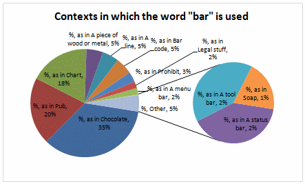
Click on the Instagram slice of the pie chart to select. To create a Pie of Pie or Bar of Pie chart follow these stepsSelect the data range in this example B5C14 On the Insert tab in the Charts group choose the Pie and Doughnut button. In that case you would add a Filter around.

Pie of Pie chart in Excel Step 1. A pie chart shows the data points of a single data series. Ad Tableau Helps People Transform Data Into Actionable Insights.

Once you have the data in place below are the steps to create a Pie chart in Excel. Afterward from the drop-down. I am working with MsXl 2010 and using a 47 numbers selected from an existing spreadsheet column the represent percentages 1-100.

To do this select a Row Labels cell or the Column Labels cell that you want to group right-click your selection and choose Group from the shortcut menu. Now in Toolbar under Design option select Change Chart Type.

Create Outstanding Pie Charts In Excel Pryor Learning